CEE-12770-Team5
12-770 Project Experiment Progress
This page documents the weekly progress of our 12-770 course project on acoustic anomaly detection for small fan and HVAC-like systems. Our work combines hardware setup, real-world audio acquisition, signal analysis, baseline model development, and interactive demo deployment.
At the current stage, the project has progressed through three major phases:
- Week 1-2: hardware setup and sensing pipeline debugging
- Week 3: signal stabilization, preliminary analysis, and baseline model training
- Week 4: demo deployment and real-world recording experiments
The long-term goal of this project is to build a practical anomaly detection pipeline that can distinguish normal and abnormal fan operating conditions from sound recordings, and later adapt the system more closely to our own physical setup through fine-tuning.
Week 1-2 – Hardware Setup and Debugging
During the first week, the main focus was on building a functional sensing pipeline using the ESP32 and the INMP441 I2S microphone. The setup involved wiring the I2S interface (WS, SCK, SD), configuring the ESP32 I2S driver, and streaming acquired data through serial communication.
Issues Encountered
Several problems were identified during the initial setup phase:
- The system repeatedly produced all-zero signal output.
- This indicated that the I2S data stream was not being received correctly.
Potential Causes Investigated
The following possible causes were tested during debugging:
- Incorrect wiring, especially mismatches among
WS,SCK, andSD - Improper
L/Rpin connection, leading to channel selection issues - Sampling rate or buffer configuration mismatch
- Serial bandwidth limitations affecting output interpretation
Debugging Process
To isolate the problem, the following steps were taken:
- Verified the wiring against the microphone datasheet
- Ensured that the
L/Rpin was fixed rather than left floating - Switched from printing raw samples to reporting aggregated amplitude values
- Adjusted sampling rate and buffer settings
- Tested different serial baud rates
Week 1-2 Outcome
By the end of Week 2, a stable data acquisition pipeline had been established, and the microphone was confirmed to output valid non-zero signals.
Week 3 – Signal Stabilization, Preliminary Analysis, and Baseline Model Training
In the second week, the project moved from hardware debugging to signal quality improvement, preliminary signal validation, and the setup of the baseline anomaly detection model. The goal was not only to confirm that the sensing system could capture meaningful differences across operating conditions, but also to begin constructing the machine-learning pipeline that will later support anomaly detection.
Key Improvement
A major issue involving distorted or difficult-to-interpret output was addressed.
- The system was modified to use window-based average amplitude rather than unstable raw sample inspection.
- This significantly improved signal stability and interpretability.
Experimental Setup
Three scenarios were recorded for comparison:
- Quiet — baseline condition with laptop background noise
- Fan at constant voltage
- Fan under varying voltage
All experiments were conducted under real-world conditions with persistent environmental noise from laptop operation.
Data Analysis
The collected data were analyzed in Python using:
- time-series plots
- rolling mean
- histogram
- boxplot
Results are shown below:
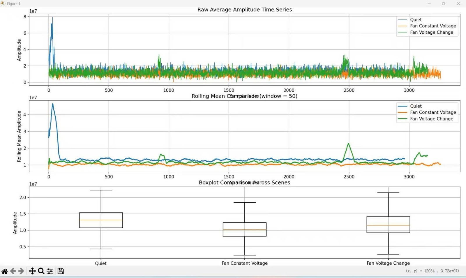
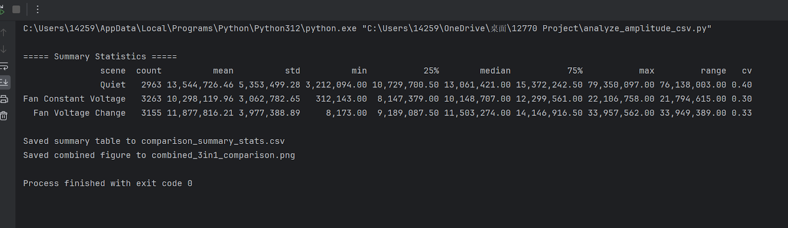
Observations
Clear separability between scenarios
- Quiet showed the highest mean amplitude and the largest variance, reflecting random ambient noise.
- Fan at constant voltage showed the lowest variance, indicating a stable mechanical operating condition.
- Fan under varying voltage showed an intermediate mean with stronger fluctuations, reflecting dynamic system behavior.
Rolling mean trends
- Fan at constant voltage exhibited a stable baseline.
- Fan under varying voltage showed visible spikes and fluctuations over time.
Distribution differences
- Fan at constant voltage had the most concentrated distribution.
- Quiet had the widest spread.
- Fan under varying voltage showed a moderate spread with noticeable spikes.
Key Insight
Even in the presence of persistent background noise, the system was able to distinguish among different operating conditions. This suggests that amplitude-based features are both robust and sensitive to mechanical state changes.
Baseline Model Training Pipeline
In parallel with signal analysis, we also established the baseline model training pipeline for acoustic anomaly detection. The objective of this stage was to convert raw audio into structured spectral features and train a reconstruction-based model that can later be used to distinguish normal and abnormal operating sounds.
Audio Preprocessing
The input .wav files are first loaded as floating-point waveforms and resampled to 16,000 Hz. This standardizes the sampling rate while preserving the dominant frequency content relevant to fan anomaly detection.
Next, Short-Time Fourier Transform (STFT) is applied with:
n_fft = 1024hop_length = 512
This transforms the waveform into a time-frequency representation, allowing the model to capture how spectral content evolves over time.
The linear-frequency spectrum is then mapped to 64 mel bands, producing a compact mel-spectrogram representation. After that, the mel-spectrogram is converted to log-mel energy, which compresses the dynamic range and improves numerical stability for learning.
Frame Stacking
Instead of using one spectral frame at a time, the model stacks 5 consecutive frames together. Since each frame contains 64 mel coefficients, this results in a 320-dimensional input vector:
64 mel coefficients × 5 frames = 320 dimensions
This step allows the model to capture short-term temporal context rather than relying only on a single instantaneous spectral snapshot.
Vector Sequence Generation
For each audio clip, frame stacking is applied in a sliding-window manner across the full signal. As a result, one audio file is converted into a sequence of 320-dimensional vectors.
This design increases the effective number of training samples and allows file-level anomaly scores to be computed by aggregating reconstruction errors across many local feature vectors.
Model Architecture
The baseline anomaly detector is implemented as a fully connected autoencoder.
Architecture
- Input Layer: 320
- Encoder: 320 -> 64 -> 64 -> 8
- Decoder: 8 -> 64 -> 64 -> 320
The hidden layers use ReLU activation functions to provide nonlinear representation power, while the output layer remains linear so that the reconstructed output can match the continuous log-mel feature space.
The 8-dimensional bottleneck layer forces the network to retain only the most salient structure of normal acoustic patterns. As a result, abnormal sounds are expected to be reconstructed less accurately.
Training Objective
The model is trained using mean squared error (MSE) between the input vector and the reconstructed output:
- lower reconstruction error indicates stronger consistency with learned normal patterns
- higher reconstruction error suggests possible abnormality
This makes MSE suitable both as the training loss and as the anomaly score during inference.
Week 3 Outcome
By the end of Week 3, the project had achieved progress on both the sensing and modeling sides:
- stabilized the signal acquisition process
- confirmed separability among multiple operating conditions
- established the baseline audio preprocessing pipeline
- implemented the baseline autoencoder architecture
- prepared the model training framework for reconstruction-based anomaly detection
Week 4 – Demo Deployment and Real-World Recording Experiments
In the third week, the project progressed from offline analysis and baseline model setup to interactive demonstration and real-world recording validation. The main focus was on building a working demo interface, testing the model with externally recorded fan sounds, and extending the system from offline uploaded-audio analysis to browser-based live microphone inference.
Demo Development
During this stage, we built an interactive demo for anomaly detection. The demo was designed to support both uploaded audio analysis and live microphone analysis using the same preprocessing and reconstruction-based inference pipeline.
The updated demo now supports:
- audio upload for offline testing
- model inference using the established autoencoder pipeline
- threshold-based prediction output
- interpretable display of reconstruction-based anomaly results
- live microphone streaming directly from the browser
- rolling-window analysis for near-real-time prediction updates
In live mode, the browser continuously streams microphone audio to the backend. Instead of analyzing each tiny chunk independently, the system maintains a rolling buffer containing the most recent 10 seconds of audio. After at least 2 seconds of signal have been accumulated, the backend begins inference and updates the prediction every 1 second. At each update, the buffered waveform is converted into stacked log-mel features and passed through the four trained models to generate anomaly scores and threshold-based decisions.
This step was important because it connected the modeling pipeline to a user-facing interface and made the anomaly detection results easier to test and interpret in practice.
Smartphone Recording Experiment
To evaluate the system under more realistic conditions, we conducted a new set of recording experiments using a smartphone microphone.
Recording Setup
The smartphone was positioned:
- 15 cm away from the fan
- at an angle of 45 degrees relative to the outlet side of the fan
Three voltage conditions were tested:
- 4 V
- 8 V
- 12 V
For each voltage level, two groups of experiments were conducted:
- Normal fan operation
- Blocked condition, in which a board higher than the fan was placed in front of it to partially obstruct the airflow during recording
Experimental Purpose
The goal of this experiment was to determine whether the system could capture meaningful acoustic differences not only across different operating voltages, but also between normal and disturbed airflow conditions.
This experiment also served as an important intermediate step between controlled baseline data and future fine-tuning on real fan recordings.
Observations from Smartphone Recordings
From the smartphone recordings, the acoustic difference between the two operating groups was clearly perceptible.
Key observations included:
- under the same voltage, the blocked fan produced a noticeably different sound pattern from the normal fan
- changes in voltage also led to audible variation in fan behavior and sound intensity
- the combination of multiple voltages and two physical operating conditions created a richer and more realistic testing set for the demo
These results suggest that the fan sound contains meaningful acoustic signatures related both to operating intensity and to physical disturbance conditions.
Real-Time Demo Experiment
In addition to offline recording tests, we further developed and tested a real-time demo workflow based on browser microphone streaming.
In this setup:
- the browser microphone was used as the live input source
- audio was continuously streamed to the backend during recording
- the backend maintained a rolling 10-second audio buffer
- the system began prediction after the first 2 seconds of signal had been collected
- the four-model inference results were refreshed every 1 second
- the live diagnostic output was displayed directly in the demo interface
This design provided a much more practical form of online anomaly monitoring than the earlier file-only workflow. Rather than waiting for a recording to finish before processing, the system could continuously evaluate the most recent segment of incoming sound and update the results interactively.
This experiment was an important step toward live anomaly detection, since it moved the system closer to practical deployment rather than relying only on pre-recorded .wav files.
Week 4 Outcome
By the end of Week 3, the project had achieved the following progress:
- built a working anomaly detection demo interface
- validated the system on smartphone-recorded fan audio
- tested multiple voltage conditions under real recording settings
- compared normal fan operation with a physically blocked condition
- confirmed that the recorded sounds show clear perceptual differences
- implemented browser-based live microphone streaming in the demo
- realized rolling-window real-time anomaly detection with periodic prediction updates
Summary of Progress So Far
Across the first three weeks, the project has achieved the following milestones:
- established a working ESP32 + INMP441 sensing pipeline
- resolved hardware-level data acquisition issues
- improved signal stability through window-based amplitude processing
- collected preliminary recordings under multiple operating conditions
- confirmed that the system can capture distinguishable patterns across different fan states
- established the baseline feature extraction and model training pipeline for acoustic anomaly detection
- built an interactive demo for reconstruction-based anomaly detection
- tested the system with smartphone-recorded fan audio under multiple voltage conditions
- implemented rolling-window live microphone analysis in the demo
Next Steps
The next phase of the project will focus on improving the connection between real-world recordings and the anomaly detection model. Planned directions include:
- collecting more real fan recordings under controlled normal and abnormal conditions
- refining the current demo workflow
- improving consistency between offline recordings and real-time inference
- fine-tuning the baseline model on target-domain normal audio
- updating thresholds after model adaptation
- preparing final report, poster, and demonstration materials
What We Learned:
Through this assignment, our team reached a strong consensus on our system architecture and experimental validation strategies. Here is what each team member learned during this phase:
Tanghao Chen:
Through deploying our Gradio-based interactive diagnostic demo, I gained a deep understanding of setting scientific decision boundaries. By analyzing validation score distributions, I configured precise MSE thresholds (e.g., 6.9, 6.0, 5.3, 7.0) for four machine IDs. A major learning point was balancing response speed and diagnostic stability during live microphone integration. I implemented a 10-second rolling buffer that accumulates 2 seconds of audio before updating predictions every second. Mastering this tradeoff between “time window length” and “interpretability” in real-time engineering was my core takeaway, laying the groundwork for future model adaptation in real physical environments.
Yizhen Xu:
My primary focus was building and training the anomaly detection models using the MIMII dataset to accurately classify the operational status of fan motors. I gained hands-on experience by implementing and comparing two distinct architectures: a baseline Dense Autoencoder (DenseAE) and a Residual Autoencoder (ResidualAE). Throughout the optimization process, I learned the critical importance of robust training strategies. I experimented with various techniques to improve model generalization, including injecting synthetic data noise, modifying the underlying network structures, and systematically tuning hyperparameters. These iterative refinements significantly deepened my understanding of autoencoder behaviors in acoustic anomaly detection.
Zexi Yin:
My key learning revolved around the complexities of real-time acoustic data acquisition. Initially building an ESP32 + INMP441 system, I spent significant time debugging issues like discontinuous signals and serial bandwidth bottlenecks at high sampling rates, eventually pivoting to SD card local storage. To ensure our demo progressed smoothly, I engineered a stable PC-based USB microphone pipeline featuring real-time recording and waveform/spectrogram visualization. Resolving buffer and shape mismatch errors taught me how to effectively manage audio data structures. Ultimately, transitioning from offline audio to window-sliced real-time streaming was a crucial structural agreement our team reached this week.